Traceability in the calibration of pressure transmitters

Traceability in the calibration of pressure transmitters

Mechanical, chemical and thermal loads over time reduce the accuracy of a pressure transmitter. For this reason they should be regularly calibrated, and it is in this context that the term “traceable” plays an important role.

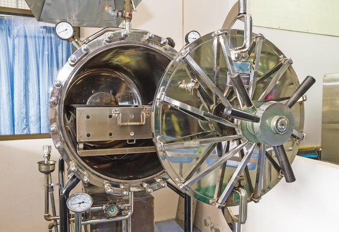
The calibration of pressure transmitters involves testing their precision and recognizing shifted readings at an early stage. A calibration thus takes place before an adjustment, during which potential malfunctions are remedied. The calibration itself is performed with the aid of a reference device (or standard). The accuracy of this reference device must be traceable to a national standard in order to meet important standards series such as EN ISO 9000 and EN 45000.

The calibration hierarchy

To ensure comparability of the measured results, these have to be traceable to a national standard via a chain of comparative measurements. If we imagine this hierarchy as a pyramid, then the accuracy will increase ascendingly. At the pinnacle stands the national standard as applied by the national institutes of metrology. In Germany, it is the Physikalisch Technische Bundesanstalt (PTB), the national testing authority, which is responsible for metrology. In the United States it is the National Institute of Standards and Technology NIST. The reference standard (also termed primary standard) is normally a deadweight tester. With a measurement uncertainty of <0.005%, this offers the greatest possible accuracy.

To fulfill its task of offering services to science and business in the field of calibration, PTB also collaborates with accredited calibration laboratories. These use factory or working standards, which are then calibrated at regular intervals with the reference standards of the national institute. Working standards reside directly below the reference standard within the hierarchy and have a typical measurement uncertainty of >0.005% to 0.05%. Factory standards, which are also applied in production with the role of quality assurance, have a typical measurement uncertainty of >0.05% to 0.6%. At the lowest level in the hierarchical structure sit the in-house testing devices

Each of these reference devices is calibrated using the next higher standard within the hierarchy. The measurement uncertainty of the standard should be three to four times lower than that of the reference device to be calibrated.

Any test equipment used internally must also be traceable to the national standard. Traceability thus describes the process by which the readings of a measuring device in one or more stages – depending on the type of device involved – can be compared with a primary standard for the relevant measured variable. The German Accreditation Body (DakkS) has defined the following elements in regard to traceability:

  1. The comparison chain must remain unbroken (by not skipping a step or comparing a test device directly with the reference standard, for example).
  2. Measurement uncertainty must be known for each step in the chain, so that the total uncertainty over the entire chain can be calculated.
  3. Every single step of the measurement chain will need to be documented.
  4. All bodies performing one or more steps in traceability must be able to demonstrate their competence by means of appropriate accreditations.
  5. The comparison chain has to end with primary standards for realizing SI units.
  6. Re-calibrations need to be carried out at regular intervals. These time periods depend on a number of factors, including the frequency and nature of use.

More detailed information on the traceability of measuring and test equipment to national standards is provided by DAkkS here.

High Accuracy Pressure Measurement at High Temperatures

High Accuracy Pressure Measurement at High Temperatures

In some applications, pressure transmitters have to work reliably when exposed to very high temperatures. Autoclaves used to sterilize equipment and supplies in the chemical and food industries are certainly one of these demanding applications.

An autoclave is a pressure chamber used in a wide range of industries for a variety of applications. They are characterized by high temperatures and pressure different from ambient air pressure. Medical autoclaves, for example, are used to sterilize equipment by destroying bacteria, viruses and fungi at 134 °C. Air trapped in the pressure chamber is removed and replaced by hot steam. The most common method for achieving this is called downward displacement: steam enters the chamber and fills the upper areas by pushing the cooler air to the bottom. There, it is evacuated through a drain that is equipped with a temperature sensor. This process stops once all air has been evacuated and the temperature inside the autoclave is 134 °C.

Very accurate measuring at high temperatures

Pressure transmitters are used in autoclaves for monitoring and validation. Since standard pressure sensors are usually calibrated at room temperature, they cannot deliver the best accuracy under the hot and wet conditions encountered in autoclaves. However, STS has recently been approached by a client in the pharmaceutical industry that requires a total error of 0,1 percent at 134 °C measuring -1 to 5 bar.

Piezoresistive pressure sensors are rather sensitive to temperature. However, temperature errors can be compensated so that the devices can be optimized for the temperatures encountered in individual applications. For example, if you use a standard pressure transmitter that achieves 0,1 percent accuracy at room temperature, the device would not be able to deliver the same degree of accuracy when used in an autoclave with temperatures of up to 134 °C.

Users who know that they require a pressure sensor that achieves a high degree of accuracy at high temperatures hence need a device that is calibrated accordingly. Calibrating a pressure sensor for certain temperature ranges is one thing. However, the client who inquired about the autoclave application with very high accuracy demands had another challenge for us that was even trickier to realize than a properly calibrated sensor: not only the sensor element was to be in the autoclave at 134 °C, but the complete transmitter including all electronics had to go in there, too. Unfortunately, we cannot go into specifics as to how we were able to assemble a digital transmitter that both delivers the desired accuracy of less than 0,1 percent total error at 134 °C but whose other components can handle the hot and moist conditions as well.

In short: Piezoresistive pressure sensors are sensitive to temperature changes. However, with the right know-how, they can be optimized for the requirements of individual applications. Moreover, not only the sensor element can be calibrated accordingly, the whole transmitter can be assembled in a way that even hot and wet conditions can be managed.

Basics of flow measurement

Basics of flow measurement

The flow of a gas or liquid is measured for a variety of reasons, certainly including commercial considerations as part of a contract and also in various production processes. The flow or volume flow (volume/time) can be recorded, among other things, by the measured value of pressure.

Volume flow can be measured using various methods. In addition to ultrasonic flow sensors, these include magnetic-inductive flow sensors and sensors that work according to the differential pressure method, among these being the orifice plate, Venturi nozzle and the Prandtl pitot tube. When evaluating the measured values, the Bernoulli equation is used for all sensors operating on the differential pressure method:

Q = V/t = VmA

Q = volume flow
Vm = median velocity
t = time
A = area
V = volume

We will now take the measurement of volume flow using an orifice plate as the example. By attaching the plate to a pipe, this then becomes narrowed at one point.

Image 1: Orifice plate

With a smooth flow, the same pressure should prevail both before and after the orifice plate:

p1 + ½ ρv12=p2+ ½ ρv22

p = pressure
ρ = density
v = velocity

This assumption is based on the continuity equation, which states that everything flowing into a pipe eventually also comes out:

v1A1 = v2A2

v = velocity

A = area

Image 2: Flow measurment

Under realistic conditions, however, friction occurs, which then leads to a pressure drop:

p + ½ ρv2 + wR = constant

p = pressure
ρ = density
v = velocity
wR = rate of frictional force by volume

Image 3: Pressure drop 

This pressure drop is important in determining the volume flow. The friction effect itself, however, depends upon many factors. For this reason, an empirical formula is used, which in turn relies on empirical values. The volume flow now ultimately results from the root of the pressure differential:

Q = 4000 αεd2√∆p/ρ

Q = volume flow
α = empirical flow coefficient
ε = expansion factor
d = internal orifice diameter
∆p = pressure differential
ρ = density

To make this formula a little easier for users, all of the constant values from the measuring system and the measuring medium can be summed up as the constant ‘c’. The result for a fluid, for example, then offers the equation:

Q = c √∆p

Pressure measurement: Compressible vs. incompressible media

Pressure measurement: Compressible vs. incompressible media

There are many factors to consider when measuring pressure. Among these, of course, are the actual properties of the medium.

One fundamental distinction is whether this is a compressible or incompressible medium. Compressible media are substances whose densities, and thus also their volumes, are pressure-dependent. This grouping applies to gases. Incompressible media, on the other hand, have a constant volume, regardless of the pressure, with liquids more likely to form part of this category. It should be noted, however, that incompressibility represents an ideal scenario that does not exist in reality. Nevertheless, liquids such as water or hydraulic oil are in practice referred to as incompressible, since they are incompressible in a first approximation. It is assumed that water inside pipelines is incompressible under normal conditions, since this simplifies calculations enormously and any resulting errors will be negligible.

An example of this is the calculation of volumetric flow. Since liquids are incompressible in a first approximation, namely their density does not change, if the cross-sectional flow is widened or narrowed at a constant volume flow (and a pressure change is thus brought about), the law of continuity then applies:

Q = A1 •v1 = A2 •v2

For gases, the law of continuity in this form does not apply due to its compressibility.

In saying this, we have slightly anticipated the next point. The distinction between statics and dynamics is also important here. Statics denotes an equilibrium of forces. In this case, no flow occurs due to the equalization of pressure differences.

Dynamics, however, is quite different. In this case, we differentiate between different types of flow.

  • Steady flow: A steady flow exists when the flow rate remains constant over time.
  •  Transient flow: A transient flow arises when temporal changes occur. This is the case with pumps and valve openings, for example. It can range from dynamic shocks to pressure spikes, which can also damage the pipes.
  • Laminar flow: In a laminar flow, the fluid flows in non-intermixing layers. There is no turbulence here and the individual layers can have different speeds.

Friction also plays a major role. A distinction is made here between outer and inner friction. The former refers to the friction that exists between the fluid and a wall (e.g., the inner wall of the conduit through which the fluid flows). An inner friction is found in the case of a laminar flow, for example, where the individual layers of fluid rub against one another. The friction that acts upon flow depends on various parameters and requires complex calculations. Those parameters include inner-wall roughness, flow velocity, density and viscosity. The latter of these also depends on temperature, which then further complicates the end calculation.

Returning now to the distinction between statics and dynamics. We speak of static pressure measurement when we seek to establish the gravitational pressure (also termed hydrostatic pressure). This refers to the pressure that arises from a still fluid under the influence of gravitational pull. Hydrostatic pressure is measured, for example, to detect the levels in tanks. Here also, the distinction between compressible and incompressible media is essential, since the calculation of the hydrostatic pressure of water, for example, is so much easier than that of a compressible gas.

The mass of incompressible media is its density times its volume, and thus the density, times the area, times the height. For the calculation of hydrostatic pressure, we use:

p = F/A = ρAhg/A = ρgh

p = pressure
F = force
A = area
ρ = density
h = height
g = gravitational force

The pressure in this equation is proportional to the depth of the medium. The shape or the cross-section of the container plays no role here. The hydrostatic pressure is thus independent of the volume within a vessel, and is instead related to the filling level. This phenomenon is also known as the hydrostatic paradox.

You can read more here about hydrostatic fill-level monitoring in tanks on a piezoresistive basis.

While static pressure is used for fill-level measurement, dynamic pressure measurements are needed to measure a volume flow or a flow quantity.You can read more about this here.

Electronic pressure measurement: Comparison of common measuring principles

Electronic pressure measurement: Comparison of common measuring principles

Electronic pressure transmitters are used in a variety of applications, from machine technology to the manufacturing sector right through to the foodstuffs and pharmaceuticals industries. The recording of the physical size of pressure can take place via different measuring principles. We introduce the common technologies here.

In electronic pressure measurement, a distinction is usually made between thin-film sensors, thick-film sensors and piezoresistive pressure sensors. It is common to all three measurement principles that the physical quantity of pressure is converted into a measurable electrical signal. Equally fundamental to all three principles is a Wheatstone bridge: a measurement device for the detection of electrical resistances, which itself consists of four interconnected resistors.

Piezoresistive pressure sensors: High-precision and cost-effective

Piezoresistive pressure sensors are based on semiconductor strain gauges made of silicon. Four resistors connected to a Wheatstone bridge are diffused onto a silicon chip. Under pressure, this silicon chip will deform and this deformation then alters the conductivity of the diffused resistors. The pressure can then ultimately be read from this shift in resistance.

Because the piezoresistive sensor element is very sensitive, it must be shielded from the influence of the measuring medium. The sensor is therefore located inside a diaphragm seal, with pressure being transmitted via a liquid surrounding the sensor element. The usual choice here is silicone oil. In hygienic applications such as in the foodstuffs or pharmaceuticals industries, however, other transfer fluids are also used. A dry measuring cell from which no liquid will escape in the event of damage is not possible.

The advantages:

  • very high sensitivity, pressures in the mbar range measurable
  • high measuring range possible, from mbar to 2,000 bar
  • very high overload safety
  • excellent accuracy of up to 0.05 percent of span
  • small sensor design
  • very good hysteresis behavior and good repeatability
  • basic technology comparatively inexpensive
  • static and dynamic pressures

The disadvantages:

Thin-film sensors: Long-term stability but expensive

In contrast to piezoresistive pressure sensors, thin-film sensors are based on a metallic main body. Upon this, the four resistors connected to a Wheatstone bridge are deposited by a so-called sputtering process. The pressure is thus detected here also by a change in resistance caused by deformation. Besides the strain gauges, temperature compensation resistors can also be inserted. A transfer liquid, as in the case of piezoresistive pressure sensors, is not necessary.

The advantages:

  • very small size
  • pressures up to 8,000 bar measurable
  • outstanding long-term stability
  • no temperature compensation required
  • high accuracy
  • high burst pressure
  • static and dynamic pressures

The disadvantages:

  • lower sensitivity than piezoresistive sensors, so low pressures are less measurable
  • basic technology comparatively expensive

Thick-film sensors: Particularly corrosion-resistant

Ceramics (alumina ceramics) serve as the basic material for thick-film sensors. These pressure sensors are monolithic, meaning that the sensor body consists of only one material, which ensures an excellent long-term stability. Furthermore, ceramics are particularly corrosion-resistant against aggressive media. With this type of sensor, the Wheatstone bridge is printed onto the main body by means of thick-film technology and then baked on at high temperature.

The advantages:

  • very good corrosion resistance
  • no temperature compensation required
  • good long-term stability
  • no diaphragm seal needed

The disadvantages:

  • not suitable for measuring dynamic pressures
  • limited upper pressure range (about 400 bar)
Correctly interpreting accuracy values for pressure sensors

Correctly interpreting accuracy values for pressure sensors

In the search for a suitable pressure transmitter, various factors will play a role. Whilst some applications require a particularly broad pressure range or an extended thermal stability, to others accuracy is decisive. The term “accuracy”, however, is defined by no standards. We provide you with an overview of the various values.

Although ‘accuracy’ is not a defined norm, it can nevertheless be verified from values relevant to accuracy, since these are defined across all standards. How these accuracy-relevant values are specified in the datasheets of various manufacturers, however, remains entirely up to them. For users, this complicates the comparison between different manufacturers. It thus comes down to how the accuracy is presented in the datasheets and interpreting this data correctly. A 0.5% error, after all, can be equally as precise as 0.1% – it’s only a question of the method adopted for determining that accuracy.

Accuracy values for pressure transmitters: An overview

The most widely applied accuracy value is non-linearity. This depicts the greatest possible deviation of the characteristic curve from a given reference line. To determine the latter, three methods are available: End Point adjustment, Best Fit Straight Line (BFSL) and Best Fit Through Zero. All of these methods lead to differing results.

The easiest method to understand is End Point adjustment. In this case, the reference line passes through the initial and end point of the characteristic curve. BSFL adjustment, on the other hand, is the method that results in the smallest error values. Here the reference line is positioned so that the maximum positive and negative deviations are equal in degree.

The Best Fit Through Zero method, in terms of results, is situated between the other two methods. Which of these methods manufacturers apply must usually be queried directly, since this information is often not noted in the datasheets. At STS, the characteristic curve according to Best Fit Through Zero adjustment is usually adopted.

The three methods in comparison:

Measurement error is the easiest value for users to understand regarding accuracy of a sensor, since it can be read directly from the characteristic curve and also contains the relevant error factors at room temperature (non-linearity, hysteresis, non-repeatability etc.). Measurement error describes the biggest deviation between the actual characteristic curve and the ideal straight line. Since measurement error returns a larger value than non-linearity, it is not often specified by manufacturers in datasheets.

Another accuracy value also applied is typical accuracy. Since individual measuring devices are not identical to one another, manufacturers state a maximum value, which will not be exceeded. The underlying “typical accuracy” will therefore not be achieved by all devices. It can be assumed, however, that the distribution of these devices corresponds to 1 sigma of the Gaussian distribution (meaning around two thirds). This also implies that one batch of the sensors is more precise than stated and another batch is less precise (although a particular maximum value will not be exceeded).

As paradoxical as it may sound, accuracy values can actually vary in accuracy. In practice, this means that a pressure sensor with 0.5% error in maximal non-linearity according to End Point adjustment is exactly as accurate as a sensor with 0.1% error of typical non-linearity according to BSFL adjustment.

Temperature error

The accuracy values of non-linearity, typical accuracy and measurement error refer to the behavior of the pressure sensor at a reference temperature, which is usually 25°C. Of course, there are also applications where very low or very high temperatures can occur. Because thermal conditions influence the precision of the sensor, the temperature error must additionally be included. More about the thermal characteristics of piezoresistive pressure sensors can be found here.

Accuracy over time: Long-term stability

The entries for accuracy in the product datasheets provide information about the instrument at the end of its production process. From this moment on, the accuracy of the device can alter. This is completely normal. The alterations over the course of the sensor’s lifetime are usually specified as long-term stability.  Here also, the data refers to laboratory or reference conditions. This means that, even in extensive tests under laboratory conditions, the stated long-term stability cannot be quantified precisely for the true operating conditions. A number of factors need to be considered: Thermal conditions, vibrations or the actual pressures to be endured influence accuracy over the product’s lifetime.

This is why we recommend testing pressure sensors once a year for compliance to their specifications. It is essential to check variations in the device in terms of accuracy. To this end, it is normally sufficient to check the zero point for changes while in an unpressurized state. Should this be greater than the manufacturer’s specifications, the unit is likely to be defective.

The accuracy of a pressure sensor can be influenced by a variety of factors. It is therefore wholly advised to consult the manufacturers beforehand: Under which conditions is the pressure transmitter to be used? What possible sources of error could occur? How can the instrument be best integrated into the application? How was the accuracy specified in the datasheet calculated? In this way, you can ultimately ensure that you as a user receive the pressure transmitter that optimally meets your requirements in terms of accuracy.

Subscribe To Our Newsletter

Join our mailing list to receive the latest news and updates from our team.

You have Successfully Subscribed!